통계적 차익거래는 움직임이 유사한 둘 이상의 자산에서 괴리가 발생하면 매수 및 매도를 통해 차익을 얻는 계량 투자 전략이다. 예를 들어 금광 채굴 회사의 주가는 금 가격과 상관성이 높을 테니, 금 가격만큼 충분히 주가가 오르지 않으면 매수하고 기다렸다가 적정 수준까지 주가가 따라잡았을 때 청산하는 식이다.
그러나 금과 금 채굴회사처럼 이미 잘 알려진 유사 자산에서 알파를 기대하긴 어렵고, 시장에서 잘 알려지지 않은 자산 쌍을 통계적으로 발굴해내야 한다. 보편적인 방법으로 K-means clustering 같은 거리 기반 비지도학습 알고리즘을 사용할 수 있다.
먼저 나스닥에 상장한 100개 자산에서 유사한 군집들을 묶고, 각 군집 내에서 상관계수가 가장 높은 쌍에 대해 차익거래 백테스팅을 수행해보자.
1. 데이터 수집
나스닥 종목 리스트로 구글링 하니 위키피디아가 검색된다.
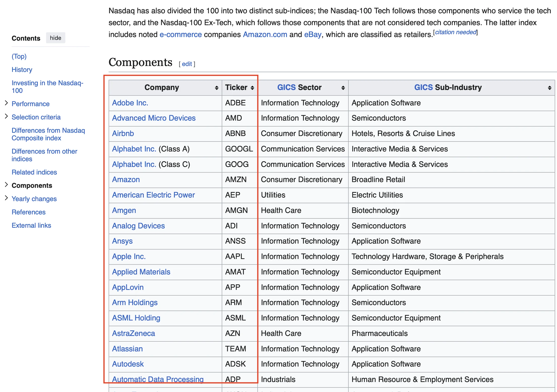
https://en.wikipedia.org/wiki/Nasdaq-100
1-1. 웹 크롤링
Ticker 목록을 크롤링하는 함수를 하나 작성해 준다.
1
2
3
4
5
6
7
8
9
10
11
12
13
14
15
16
17
18
# Get NASDAQ-100 tickers using Wikipedia
import requests
from bs4 import BeautifulSoup

def get_nasdaq100_tickers():
    url = "https://en.wikipedia.org/wiki/Nasdaq-100"
    response = requests.get(url)
    soup = BeautifulSoup(response.text, 'html.parser')

    # Find the table with Nasdaq-100 components
    tables = soup.find_all('table', {'class': 'wikitable'})
    for table in tables:
        if 'Ticker' in str(table):
            df = pd.read_html(str(table))[0]
            # Get the ticker column (may need adjustment based on Wikipedia table structure)
            tickers = df['Ticker'].tolist()
            return tickers
    return []
1-2. yfinance
함수로 Ticker 목록을 가져온 다음, Ticker를 순회하며 야후 파이낸스 api로 실제 주가 데이터를 수집한다.
1
2
3
4
5
6
7
8
9
10
11
12
13
14
15
16
17
18
19
20
21
22
23
# Get NASDAQ-100 tickers
nasdaq100_tickers = get_nasdaq100_tickers()

# Get NASDAQ composite index data
nasdaq = yf.Ticker("^IXIC")
nasdaq_data = nasdaq.history(period="5y")

# Download historical data for all NASDAQ-100 stocks
stock_data = {}
print("Downloading data for NASDAQ-100 stocks...")

for ticker in nasdaq100_tickers:
    try:
        stock = yf.Ticker(ticker)
        data = stock.history(period="5y")['Close']
        if not data.empty:
            stock_data[ticker] = data
            print(f"Downloaded {ticker}")
    except Exception as e:
        print(f"Error downloading {ticker}: {e}")

 prices = pd.DataFrame(stock_data)
 returns = prices.pct_change() # daily returns
2. Clustering(군집 분석)
2-1. 최적의 군집 수 찾기
주가 데이터를 각 움직임 특성에 따라 N개 그룹으로 구분하고자 한다. N을 지정해야 하는데, 임의로 지정하기보다 최적의 N을 찾는 elbow method를 사용하겠다. elbow method는 각 군집 내 요소들에 대해 속한 군집의 중심으로부터 거리 합을 계산하여 그 값이 최소 혹은 충분히 낮은 수준으로 떨어지는 군집의 수를 찾는 방법론이다.
1
2
3
4
5
6
7
8
9
10
11
12
13
14
15
16
17
18
19
20
21
# Normalize prices to start at 100 for fair comparison
from sklearn.cluster import KMeans
normalized_prices = complete_prices / complete_prices.iloc[0] * 100

# Determine optimal number of clusters using elbow method
inertias = []
K = range(1, 11)

for k in K:
    kmeans = KMeans(n_clusters=k, random_state=42)
    kmeans.fit(normalized_prices.T)  # Transpose to cluster stocks, not timestamps
    inertias.append(kmeans.inertia_)

# Plot elbow curve
plt.figure(figsize=(12, 6))
plt.plot(K, inertias, 'bx-')
plt.xlabel('k')
plt.ylabel('Inertia')
plt.title('Elbow Method For Optimal k')
plt.grid(True)
plt.show()
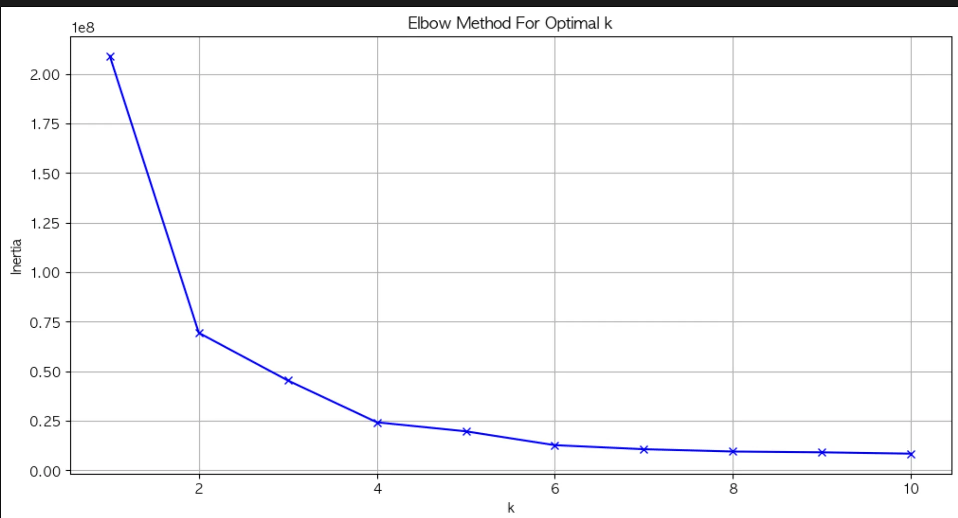
군집의 수가 늘어날수록 중심으로부터의 거리 합이 작아지는데, 그렇다고 군집을 수치에 따라 무한정 늘리면 군집 내 요소가 하나, 둘 수준으로 과하게 적게 포함되어 그룹으로 묶겠다는 의도를 제대로 반영할 수 없다. 따라서 충분히 낮은 수치를 만드는 구간인 6이 군집의 수로 적당하다.
2-2. 유사 자산 그룹 묶기
1
2
3
4
5
6
7
8
9
10
11
12
13
14
15
16
17
18
19
20
21
22
23
24
25
26
27
28
29
30
31
32
33
34
# Choose optimal k (let's use 4 clusters) and perform final clustering
optimal_k = 6
kmeans = KMeans(n_clusters=optimal_k, random_state=42)
clusters = kmeans.fit_predict(normalized_prices.T)

# Plot clusters
plt.figure(figsize=(15, 8))
for i in range(optimal_k):
    # Get tickers in this cluster
    cluster_tickers = normalized_prices.columns[clusters == i]

    # Plot mean trajectory of cluster
    cluster_mean = normalized_prices[cluster_tickers].mean(axis=1)
    plt.plot(normalized_prices.index, cluster_mean, linewidth=2, label=f'Cluster {i+1}')

    # Print cluster members and count
    print(f"\nCluster {i+1} members ({len(cluster_tickers)} stocks):")
    print(', '.join(cluster_tickers))

plt.title('Stock Price Clusters (Common Period Only)')
plt.xlabel('Date')
plt.ylabel('Normalized Price')
plt.legend()
plt.grid(True)
plt.show()

# Print summary statistics for each cluster
print("\nCluster Summary Statistics:")
for i in range(optimal_k):
    cluster_tickers = normalized_prices.columns[clusters == i]
    cluster_returns = returns.loc[valid_dates, cluster_tickers].mean(axis=1)
    print(f"\nCluster {i+1}:")
    print(f"Average Return: {cluster_returns.mean():.4f}")
    print(f"Return Std Dev: {cluster_returns.std():.4f}")
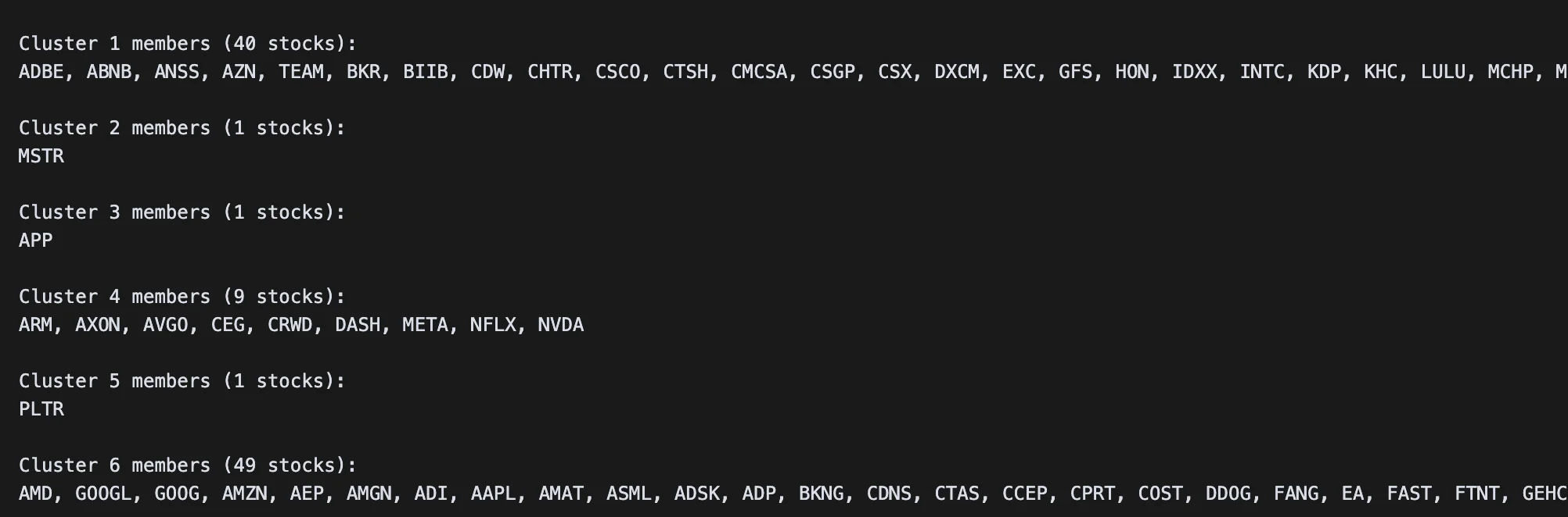
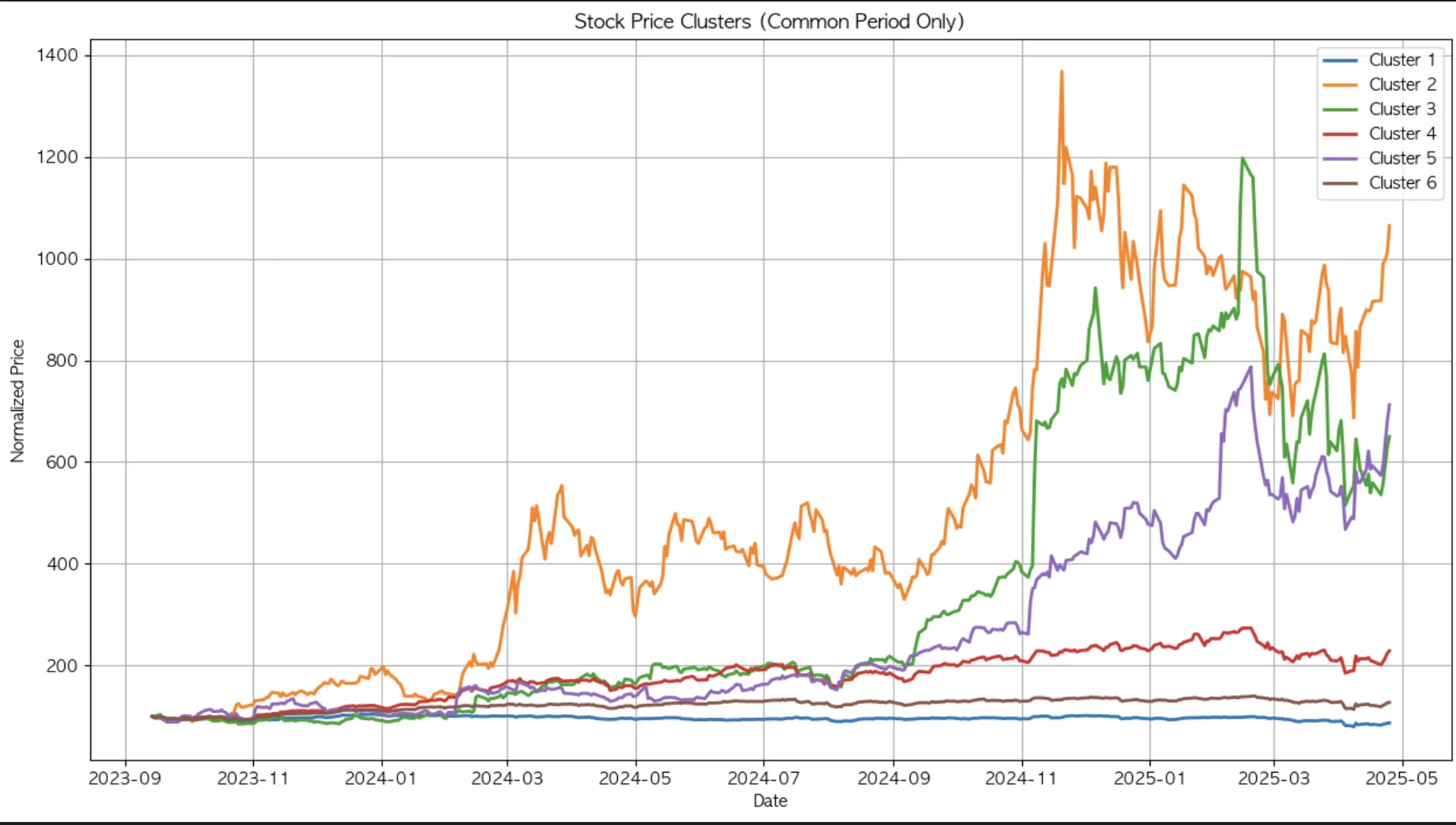
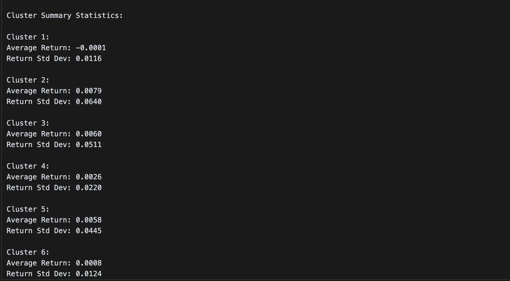
많지 않은 군집 수로 클러스터링을 수행했음에도 자산이 하나씩만 포함된 군집이 3개나 존재한다. 다른 자산들과 묶이기에는 움직임 특성에 뚜렷한 차이가 있는 것이다. 특히 5번 클러스터에 묶인 팔란티어 같은 경우 다른 군집과 다소 상이한 움직임을 보이고 있다.
3. 차익거래 백테스팅
우리는 각 군집 내에서 상관관계가 높은 쌍을 찾아야 하므로, 클러스터 내 요소 수가 하나인 경우 제외하고 1번, 4번, 6번 클러스터만 분석에 활용한다.
1
2
3
4
5
6
7
8
9
10
11
12
13
14
15
16
17
18
19
20
21
22
23
24
25
26
27
28
29
30
31
32
33
34
35
36
37
38
39
40
41
42
43
44
45
46
47
48
49
50
51
52
53
54
55
56
57
58
59
60
61
62
63
64
65
66
67
68
69
70
71
72
73
74
75
76
77
78
79
80
81
82
83
84
85
86
87
88
89
90
91
92
93
94
95
96
97
98
99
100
101
102
103
104
105
106
107
selected_clusters = [0, 3, 5]

# Dictionary to store results
pair_trading_results = {}

for cluster_idx in selected_clusters:
    print(f"\nAnalyzing Cluster {cluster_idx + 1}")

    # Get tickers in this cluster
    cluster_tickers = normalized_prices.columns[clusters == cluster_idx]
    cluster_prices = normalized_prices[cluster_tickers]

    # Calculate all possible pairs in the cluster
    pairs = []
    correlations = []
    for i in range(len(cluster_tickers)):
        for j in range(i+1, len(cluster_tickers)):
            stock1, stock2 = cluster_tickers[i], cluster_tickers[j]
            correlation = cluster_prices[stock1].corr(cluster_prices[stock2])
            pairs.append((stock1, stock2))
            correlations.append(correlation)

    # Select the pair with highest correlation
    best_pair_idx = np.argmax(correlations)
    stock1, stock2 = pairs[best_pair_idx]
    correlation = correlations[best_pair_idx]

    print(f"Best pair: {stock1} - {stock2} (correlation: {correlation:.4f})")

    # Calculate spread
    spread = cluster_prices[stock1] - cluster_prices[stock2]

    # Calculate z-score of spread
    z_score = (spread - spread.mean()) / spread.std()

    # Define trading signals
    entry_threshold = 2.0  # Enter position when |z-score| > 2
    exit_threshold = 0.0   # Exit position when z-score crosses 0

    # Initialize position and returns arrays
    position = np.zeros(len(z_score))
    returns = np.zeros(len(z_score))

    # Implement trading strategy
    for i in range(1, len(z_score)):
        # If no position is open
        if position[i-1] == 0:
            if z_score[i] > entry_threshold:
                position[i] = -1  # Short stock1, long stock2
            elif z_score[i] < -entry_threshold:
                position[i] = 1   # Long stock1, short stock2
        # If position is open
        else:
            if (position[i-1] == 1 and z_score[i] > exit_threshold) or \
               (position[i-1] == -1 and z_score[i] < exit_threshold):
                position[i] = 0   # Close position
            else:
                position[i] = position[i-1]  # Maintain position

        # Calculate returns
        if position[i] != 0:
            stock1_return = (cluster_prices[stock1].iloc[i] / cluster_prices[stock1].iloc[i-1] - 1)
            stock2_return = (cluster_prices[stock2].iloc[i] / cluster_prices[stock2].iloc[i-1] - 1)
            returns[i] = position[i] * (stock1_return - stock2_return)

    # Calculate strategy metrics
    cumulative_returns = np.cumprod(1 + returns) - 1
    sharpe_ratio = np.sqrt(252) * returns.mean() / returns.std()

    # Store results
    pair_trading_results[f"Cluster_{cluster_idx + 1}"] = {
        'pair': (stock1, stock2),
        'correlation': correlation,
        'cumulative_returns': cumulative_returns,
        'sharpe_ratio': sharpe_ratio
    }

    # Plot results
    plt.figure(figsize=(15, 10))

    plt.subplot(2, 1, 1)
    plt.plot(cluster_prices.index, z_score)
    plt.axhline(y=entry_threshold, color='r', linestyle='--')
    plt.axhline(y=-entry_threshold, color='r', linestyle='--')
    plt.axhline(y=0, color='k', linestyle='-')
    plt.title(f'Z-Score of Spread ({stock1} - {stock2})')
    plt.grid(True)

    plt.subplot(2, 1, 2)
    plt.plot(cluster_prices.index, cumulative_returns)
    plt.title('Cumulative Returns')
    plt.grid(True)

    plt.tight_layout()
    plt.show()

    print(f"Sharpe Ratio: {sharpe_ratio:.2f}")
    print(f"Total Return: {cumulative_returns[-1]:.2%}")

# Print overall summary
print("\nOverall Strategy Summary:")
for cluster, results in pair_trading_results.items():
    print(f"\n{cluster}:")
    print(f"Pair: {results['pair'][0]} - {results['pair'][1]}")
    print(f"Correlation: {results['correlation']:.4f}")
    print(f"Sharpe Ratio: {results['sharpe_ratio']:.2f}")
    print(f"Total Return: {results['cumulative_returns'][-1]:.2%}")
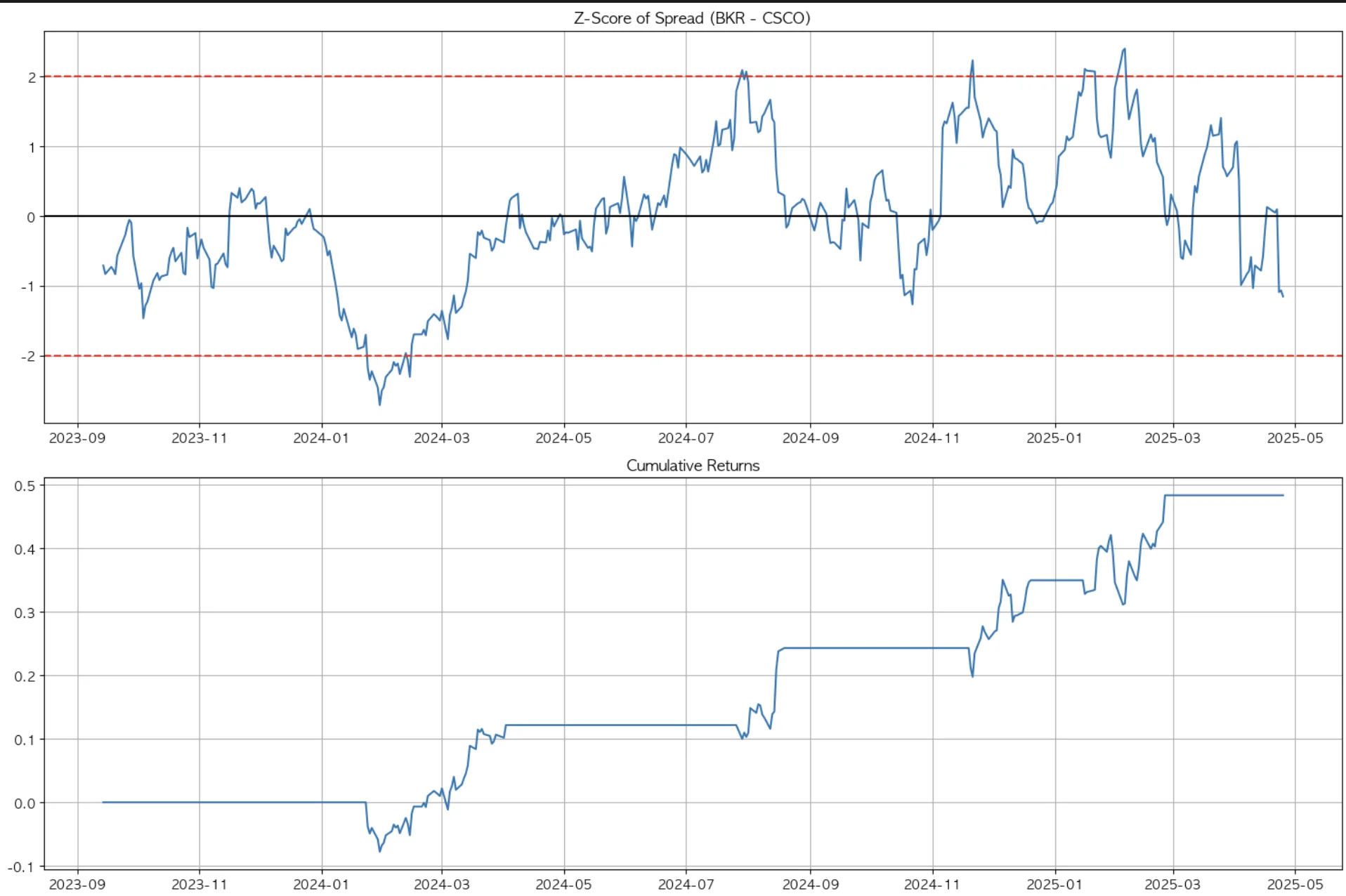
각 군집별 최적의 쌍을 찾고, 둘의 스프레드가 2 표준편차를 벗어나면 가격이 높은 자산은 매도하고 낮은 자산은 매수하도록 했다.
3-1. Baker Hughes & Cisco
첫 번째 군집에서는 BKR과 CSCO가 상관계수 89%로 움직임이 가장 유사했는데, long-short 전략을 수행했을 때 2년이 안 되는 기간 동안 약 48%의 수익률을 보였다. sharpe ratio 역시 1.8로 매우 우수한 수준이다.

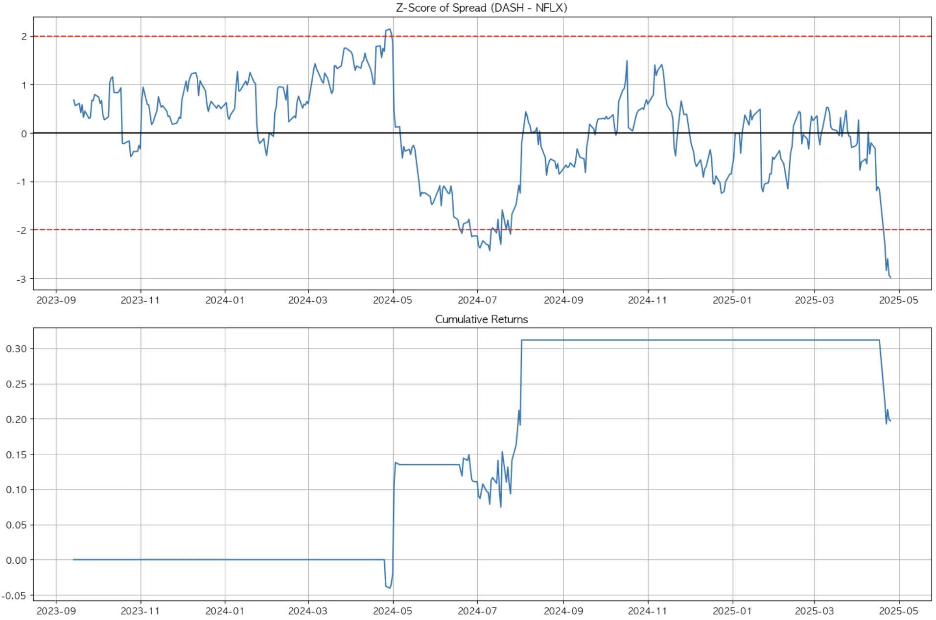
3-2. Door Dash & Netflix
이어서 도어대시와 넷플릭스는 상관계수 96%로 첫 번째 그룹보다 높은 상관성을 보인다. 그러나 상관성이 높다고 차익거래 성과가 더 좋은 것은 아니다.
오히려 스프레드 변동성이 낮고, 스프레드 발생 구간이 짧아 트레이딩 효용은 떨어진다. 또, 최근 발생한 스프레드에 대해 수익이 발생하려면 스프레드 내구간으로 재진입해야 하나 아직 그 시점이 오지 않아 손실이 발생하고 있는 것을 감안해야 한다.

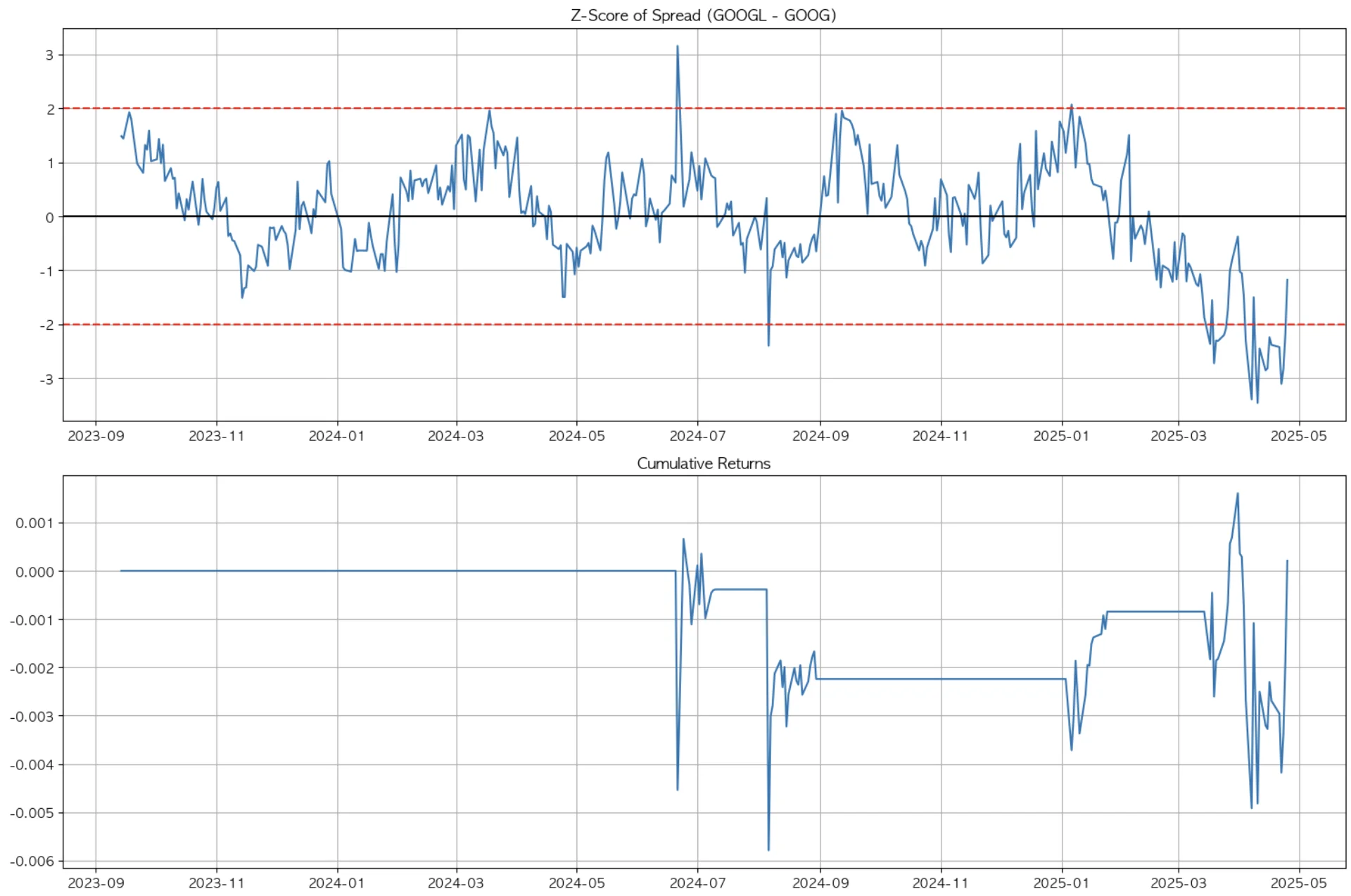
3-3. GOOG & GOOGL
한국으로 치면 보통주, 우선주 개념의 의결권 차이만 있을 뿐 둘은 사실상 같은 구글 주식이다. 당연히 상관계수는 99%로 가장 높고, 여기서 알파는 찾을 수 없었다. sharpe ratio도 낮고 return은 시장 수익률에 미치지 못했다.
알려진 시장은 효율적이고, 서두에서 언급했듯 누구나 동일 혹은 유사 자산으로 인지할 수 있는 자산 쌍에 대해서는 차익거래를 통한 수익을 취할 수 없다.

이렇게 파이썬으로 간단히 통계적 차익거래를 시뮬레이션해 보았다. 자산 움직임에 따른 유사 군집으로 먼저 타겟 집단을 좁히고, 타겟 집단 내에서 상관계수가 가장 높은 쌍을 찾아 해당 자산 쌍에 대해 long-short 매매를 진행했을 때 스프레드 변동성이 크고 잦은 Baker Hughes & Cisco에서 가장 높은 수익률을 확인할 수 있었다.
자동매매가 판치는 자산 시장에서도 찰나 혹은 꽤나 긴 시간 동안 비효율은 발생할 수 있으며, 시장 국면에 따라 이러한 비효율을 발굴하여 상관계수가 높은 자산 쌍을 타겟으로 차익거래를 시도해 볼 수 있다.
관성을 이기는 데이터